As I mentioned in the post 3, about the "speculators" they apply an optimal adjustment back-office method that multiplies their profits reduces the risk, and does not need a forecasting of the market. Warren Buffett and many other successful investors apply this technique as a paramount and basic necessity in investing and trading.
During 1998 while studying in the University of Portsmouth, I discovered a theorem in the book "Stochastic Differential equations" by B. K. Oksendal (Springer editions) page 223, example 11.5 where he proves through the ITO stochastic calculus that such an adjustment as above is optimal during a constant trend ( so only the buy-and-hold is not the optimal) , and maximizes the logarithm of the average wealth at the end of a time interval (using the Kelly criterion, a logarithmic utility function of the wealth ). In fact it gives also an optimal formula of how much the tradable funds should be compared to the non-tradable by tradable funds percentage=(r-r0)/ s^2 if it is less than 1. Where r is the rate of return of the constant trend, or drift, r0 is the bank's risk free rate, and s^2 is the variance of the rate of return of the trend (some times referred also as volatility of the trend). But in practice investors just use the value 2/3 or 66% . The traders should adjust this value of 66% for a more optimal with extended many years back-tests.
We may apply the above theorem and technique of adjustments not to a particular trend of the market but rather to the rather constant trend of the equity curve of a successful trading system.
This means that we divide the funds in to tradable (e.g. 66%) and non-tradable (33%). All trading is based only on the tradable funds, which in their turn are divided in to usable for margin, and risked e.g. by stop-loss in a trade or excursions, and those reserved for next trades. Then at the start of the trading we mark the equity level E0. For every dE increase from this E0 level or previous level during trading (e.g. dE=5% over all funds) or alternatively every equal time intervals, we adjust by in increasing by 2.5% the non-tradable, and decreasing by 2.5% the tradable, and for every dE decrease from E0 or previous level during trading, we adjust by in decreasing by 2.5% the non-tradable, and increasing by 2.5% the tradable so that the ratio 33% of non-tradable funds to all funds, remains approximately constant. From the non-tradable cash we may withdraw periodically in equal time intervals, so withdrawals are involved also in the optimal adjustments and trading, through the above constant ratio of 33%.
The optimal adjustment is not to be confused with the re-investment technique and the Kelly formula.
There is also a corresponding continuous time theory about the risks of bankruptcy of a constant exponential trend (or drift ) r equity curve, with standard deviation s of it. An exponentially growing equity curve is when the trading is under reinvestment (money management)
(see e.g. http://users.softlab.ece.ntua.gr/~kyritsis/PapersInEconomics/KICHOS6.htm )
A simple formula is that if r<(1/2)*(s^2) then an account crash will occur with probability equal to 1 (almost certainly). To avoid a crash of the account it must hold that r>>(1/2)*(s^2).
Also in the book "A first course in Stochastic Processes" by Samuel Karlin and Howard Taylor Academic Press 1975, Chapter 7 (Brownian Motion), it is proved in Theorem 5.2 p 361, that if we model the equity curve Eq(t) as Brownian Motion with drift r, and variance s^2 (or Wienner process), (notice that this means that we have not included re-investment money management), then the absolute draw down ADD=Eq(0)-minimum(Eq(t)) , for all t, follows the exponential distribution
Probability{ADD>=w}=exp(-L*w) , w>=0 , where L=2*(Absolute_value(r))/s^2
As L is also the average value of the exponential distribution, this proves that the average absolute (starting) draw down of the equity curve is equal to (s^2)/2*|r|
The larger the variance of the equity curve, the larger of the average absolute draw down, and the less the slope (drift) of the equity curve the larger the average absolute draw down.
(See also http://users.softlab.ece.ntua.gr/~kyritsis/PapersInEconomics/MLpaper2.htm )
The exponential distribution has a density as in the figure below
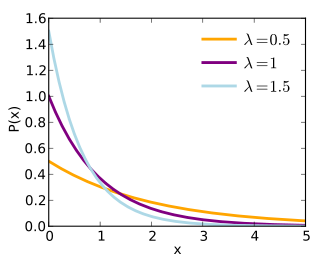
and a formula
Its average value is 1/λ.
Conversely, this formula can be utilized o make crude estimation of the variance of the rate of return in backtests: If say the rate of return in a backtest is r, and the maximum Draw Down is D, then the standard deviations s and variance s^2 of r may be estimated from d=(s^2)/2r thus s^2=2rD.
Important Remark: Because the above formulae in the statistical books, have been derived with the assumption of continuous time, continuous subdivision of the funds, and constant succes rate of trades (percentage of winning tardes) while in practice there is a minimum of lot size, and rather variable success rate of the trades, considerable deviations towards less risk should be utilized (e.g. for the Kelly percentage only 5%-25% of it as my experiments show).
The previous considerations lead to a withdrwal rule that e.g. has been applied for many years by professor Michael LeBoeuf in his investments (see https://en.wikipedia.org/wiki/Michael_LeBoeuf and http://www.nightingale.com/beat-time-money-trap-mp3.html )
CONSTANT RATIO WITHDRAWAL RULE . We may divide the funds to 2/3 of them that we trade, and 1/3 that we do not trade. The exact percentage should be defined by the ratio (f=R/a^2) (that we mention above from the book "Stochastic Differential equations" by B. K. Oksendal (Springer editions) page 223, example 11.5) where R is the average per period rate o return of the trading on the used funds, measured on a sample of periods and a^2 is the variance of this rate of return on this sample of periods. E.g. of the rate of return is 10% per period and the standard deviation a of it is 34%, then the percentage f is 2/3. Each period we re-adjust the total funds so that this ratio f applies as division of the funds. As the sample of measurement of this ratio is not small, usually it remains rather constant. We withdraw e.g. from the 1/3 non-trading funds ,each period never more than half of the average profits per period of the other 2/3 of the funds that are traded.
The above is the back office method to implement the constant ratio optimal adjustment technique. There is also the front office method, where what is kept constant is the percentage of the funds risked at each trade and in all open trades simultaneously. To implement the optimal adjustment in this way it is required an automated grid trading, where trades are opened in backwards and forwards movements of the prices and are closed by trailing-out and/or take-profits.
The combination of optimal adjusting and pyramiding, boosts the performance of classical trading by a factor of about 7 times! (See also post 32)
( The reason it is boosted so much is similar to the reason that the measurement of the periphery of an island is boosted very much if we utilze fractals to measure it, instead of visible smooth curves on the map. This is also the reason that some traders consider it the "holy grail" of trading as it converts the wealth creation by classical investment and trading that requires initial capital, to wealth creation without initial capital.)
The optimal adjustment is not to be confused with the re-investment technique and the Kelly formula.
There is also a corresponding continuous time theory about the risks of bankruptcy of a constant exponential trend (or drift ) r equity curve, with standard deviation s of it. An exponentially growing equity curve is when the trading is under reinvestment (money management)
(see e.g. http://users.softlab.ece.ntua.gr/~kyritsis/PapersInEconomics/KICHOS6.htm )
A simple formula is that if r<(1/2)*(s^2) then an account crash will occur with probability equal to 1 (almost certainly). To avoid a crash of the account it must hold that r>>(1/2)*(s^2).
Also in the book "A first course in Stochastic Processes" by Samuel Karlin and Howard Taylor Academic Press 1975, Chapter 7 (Brownian Motion), it is proved in Theorem 5.2 p 361, that if we model the equity curve Eq(t) as Brownian Motion with drift r, and variance s^2 (or Wienner process), (notice that this means that we have not included re-investment money management), then the absolute draw down ADD=Eq(0)-minimum(Eq(t)) , for all t, follows the exponential distribution
Probability{ADD>=w}=exp(-L*w) , w>=0 , where L=2*(Absolute_value(r))/s^2
As L is also the average value of the exponential distribution, this proves that the average absolute (starting) draw down of the equity curve is equal to (s^2)/2*|r|
The larger the variance of the equity curve, the larger of the average absolute draw down, and the less the slope (drift) of the equity curve the larger the average absolute draw down.
(See also http://users.softlab.ece.ntua.gr/~kyritsis/PapersInEconomics/MLpaper2.htm )
The exponential distribution has a density as in the figure below
and a formula
Its average value is 1/λ.
Conversely, this formula can be utilized o make crude estimation of the variance of the rate of return in backtests: If say the rate of return in a backtest is r, and the maximum Draw Down is D, then the standard deviations s and variance s^2 of r may be estimated from d=(s^2)/2r thus s^2=2rD.
Important Remark: Because the above formulae in the statistical books, have been derived with the assumption of continuous time, continuous subdivision of the funds, and constant succes rate of trades (percentage of winning tardes) while in practice there is a minimum of lot size, and rather variable success rate of the trades, considerable deviations towards less risk should be utilized (e.g. for the Kelly percentage only 5%-25% of it as my experiments show).
The previous considerations lead to a withdrwal rule that e.g. has been applied for many years by professor Michael LeBoeuf in his investments (see https://en.wikipedia.org/wiki/Michael_LeBoeuf and http://www.nightingale.com/beat-time-money-trap-mp3.html )
CONSTANT RATIO WITHDRAWAL RULE . We may divide the funds to 2/3 of them that we trade, and 1/3 that we do not trade. The exact percentage should be defined by the ratio (f=R/a^2) (that we mention above from the book "Stochastic Differential equations" by B. K. Oksendal (Springer editions) page 223, example 11.5) where R is the average per period rate o return of the trading on the used funds, measured on a sample of periods and a^2 is the variance of this rate of return on this sample of periods. E.g. of the rate of return is 10% per period and the standard deviation a of it is 34%, then the percentage f is 2/3. Each period we re-adjust the total funds so that this ratio f applies as division of the funds. As the sample of measurement of this ratio is not small, usually it remains rather constant. We withdraw e.g. from the 1/3 non-trading funds ,each period never more than half of the average profits per period of the other 2/3 of the funds that are traded.
No comments:
New comments are not allowed.